Cheaply improving text-image retrieval via text-encoder adaptation
How much, and how cheaply, can we improve text-image retrieval (where we use text to retrieve images), when using embedding models such as OpenAI-CLIP and SigLIP2?
I fine-tuned only the text encoders using roughly 16k external images from LAION-400M, paired with generated labels designed for retrieval. Across four models and three test datasets, fine-tuning improved mean average precision (mAP) by 4.0 points over the published prompting recipes. The evaluation covers more than 1,300 category queries. For context, switching from OpenClip-400M to OpenClip-2B (trained on 400M and 2B image–text pairs, respectively) improves mAP by 3.5 points on the same benchmarks. The caveat is that these gains are for category search using short, disambiguated object names.
CLIP's sensitivity to query wording motivates this approach: retrieval accuracy can vary widely with query wording, even when the image embeddings stay fixed [1] [11]. This suggests adapting the text encoder could improve retrieval substantially on top of fixed representations. [10] Keeping the image encoder fixed reduces deployment costs: improvements to the query encoder can be used without recomputing embeddings for the existing image collection. The gains from this light-weight fine-tuning of the text encoder exceed the gains from different prompting recipes substantially and are more consistent, as I show later in Table 1.
Below, I examine the main results, the effect of caption style, the marginal value of more training data, and possible explanations for the gains and plateaus.
Main result: Text-encoder fine-tuning improves category retrieval across models and datasets
Quick Background
CLIP (contrastive language–image pre-training) learns to map images and text into a shared vector space, allowing text queries to retrieve images. Its successors SigLIP [5] and SigLIP2 [6] provide vision encoders for VLMs such as Gemma 3 and Qwen3-VL. LAION [4] is an open collection of image–text pairs gathered from the web, using images and their associated alt text. OpenClip-400M was trained on LAION-400M, and OpenClip-2B on the larger LAION-2B.
Each model has separate image and text encoders. Images are embedded when added to the collection; at search time, the text encoder maps the query into the same space.
Method details
The recipe is straightforward: sample images from LAION-400M and generate short object labels that resolve ambiguous names. For example, “musical keyboard” or “keyboard (musical instrument)” distinguishes the instrument from a computer keyboard. Use these image–text pairs to fine-tune only the text encoder with LoRA (low-rank adaptation) [3], keeping the image encoder fixed. The resulting text encoder can then search the existing image index without re-embedding the images. Further details below.
Evaluation details
I use the same random sample from LAION-400M for all four models: 16k images for fine-tuning and 2k for validation. The models are OpenAI-CLIP, OpenClip-400M, OpenClip-2B and SigLIP2. Instead of using LAION-400M’s original text, I used GPT-4.1 mini to generate short, qualified object labels for the images. I wanted to test whether changing the training text could improve retrieval even when the images came from a dataset already used to train the model, as with OpenClip-400M. The exact captioning style matters, and I expand on that in “What should the training captions look like?”. The goal of training several model variants is to show the effect persists across different models, including SigLIP2 with much higher starting baseline quality. None of the models is fine-tuned on images from the evaluation datasets. Each model is fine-tuned once on the LAION sample, then evaluated on all three datasets without further adaptation. Later experiments show that much smaller training sets also improve retrieval, with diminishing gains as the dataset grows; see the scaling experiments. Further fine-tuning on queries and images from the target collection could yield additional gains. That is a separate direction worth exploring in practice.
Query wording affects the resulting vector. For each model, I compare its published prompting recipe with using the category name directly. The "Prompt recipe" column in Table 1 follows the reference recipe for each model. The final column shows each fine-tuned model’s results using the category name directly as its query. For each category query, I rank images and calculate AP from their relevant/irrelevant labels.
The takeaways from Table 1:
Text encoder fine-tuning improves beyond both the plain-noun baseline and the reference prompting recipe in all 12 model/dataset combinations. The largest gains are on LVIS: +4.8 to +9.7 mAP points over the prompting baseline. LVIS tests roughly 1,000 category queries, compared with roughly 300 for ObjectNet and 10 for BDD. I give its results more weight as evidence of breadth, although all three datasets are weighted equally in the headline average. In particular, the prompting recipes are inconsistent in their effects on different datasets and models.
Text-encoder fine-tuning offers a gain comparable to switching base models. With qualified-noun queries, moving from OpenClip-400M to OpenClip-2B raises mAP by 3.5 points on average across ObjectNet, LVIS and BDD. Fine-tuning OpenClip-400M’s text encoder improves mAP by 3.4 points across the same datasets, while keeping its image embeddings fixed.
Text-encoder fine-tuning stacks on top of stronger base models. Fine-tuning also improves OpenClip-2B and SigLIP2, despite their stronger starting performance. This suggests lightweight text adaptation remains useful even with stronger base models.
See the collapsible Table 1 protocol below for training settings, prompting recipes and evaluation details.
Table 1. Category retrieval mAP (%) across datasets and models. Parentheses on the right show gains from fine-tuning over the published prompt recipe, in mAP percentage points. The average row at the bottom weights all 12 model/dataset comparisons equally. The fine-tuned model beats its baseline consistently but by different degrees depending on dataset and base model.
| Dataset | Model | Category name as prompt | Published prompt recipe | Fine-tuned ( and delta ) |
|---|---|---|---|---|
| ObjectNet 313 queries 50,273 images | OpenAI-CLIP | 24.5 | 25.0 | 27.8 (+2.7) |
| OpenClip-400M | 25.2 | 24.0 | 26.7 (+2.7) | |
| OpenClip-2B | 32.1 | 30.5 | 33.7 (+3.2) | |
| SigLIP2 | 57.0 | 56.5 | 59.0 (+2.5) | |
| LVIS validation 1,002 queries 19,809 images | OpenAI-CLIP | 52.2 | 54.2 | 63.9 (+9.7) |
| OpenClip-400M | 53.0 | 50.8 | 58.8 (+7.9) | |
| OpenClip-2B | 55.1 | 53.0 | 61.5 (+8.5) | |
| SigLIP2 | 66.4 | 64.6 | 69.4 (+4.8) | |
| BDD validation objects 10 queries 10,000 images | OpenAI-CLIP | 40.1 | 42.4 | 44.4 (+2.0) |
| OpenClip-400M | 35.4 | 37.8 | 38.3 (+0.5) | |
| OpenClip-2B | 36.7 | 39.2 | 41.1 (+1.9) | |
| SigLIP2 | 45.7 | 44.3 | 46.3 (+1.9) | |
| Average (12 comparisons) | 43.6 | 43.5 | 47.6 (+4.0) | |
Table 1: training and evaluation protocol
Prompting recipes OpenAI-CLIP uses the seven-template subset selected on ImageNet [2], which includes a bad photo of the {category}. and a photo of the small {category}.. Each template produces a query vector; I average and normalize those vectors to obtain one search query. Both OpenClip variants use the 80-template ImageNet ensemble [8], and SigLIP2 uses the single template this is a photo of {category}., following its reference inference recipe [9]. For the ensembles, I normalize each text vector, average the vectors equally, and normalize the mean. For the fine-tuned model variant I only use the qualified noun variant.
Evaluation datasets ObjectNet uses all 50,273 test images and 313 category queries. LVIS uses its official 19,809-image validation split: each category is ranked only within its judged subset of visible positives and explicitly known negatives. Because CLIP preprocessing crops to a square, I also exclude positive pairs whose annotated objects are truncated by that crop. After these restrictions, 1,002 of the 1,203 LVIS categories have at least one positive and one negative image and are included in mAP. BDD uses the official 10,000-image validation split and all 10 of its object categories.
Validation metric. For each validation caption, I rank the 2k validation images and record the reciprocal rank of its designated matching image. A match in third position scores 1/3. Averaging these scores across captions gives mean reciprocal rank (MRR), which I use to select the training checkpoint.
Training settings. All four models in Table 1 use 16k training images and 2k validation images. I train small adapters using LoRA (low-rank adaptation), keeping the original model weights frozen. The adapters cover the text encoder’s attention and feed-forward layers plus its output projection. Settings are rank 64, alpha 128, batch size 4,096, dropout 0.05 and weight decay 0.01. AdamW uses a learning rate of 10⁻⁴ for adapters and 10⁻⁵ for the learned score scale and bias. These settings are not necessarily optimal.
Training objective. All four models use the pairwise logistic (sigmoid) loss from SigLIP. [5] Each score is a scaled cosine similarity plus a learned bias. Matching image–text pairs are positive examples; other image–text combinations in the batch are treated as negatives. The loss scores each pair independently, without a softmax over the batch. In this implementation, pair losses are summed over image candidates and averaged over text queries.
How much does category wording matter?
Before comparing training caption styles, how much can we gain simply by clarifying the category name used as a query? After inspecting poorly performing ObjectNet searches, I revised 76 of its 313 category names, for example changing “battery” to “electrical battery” and “button” to “clothing button”. The wording revisions were informed by inspection of ObjectNet positives, since ObjectNet does not define the categories clearly. The comparison below uses frozen OpenAI-CLIP with one category-name query, keeping the images, relevance labels and AP calculation fixed.
| Dataset | Names changed | Original names mAP (%) | Reviewed names mAP (%) | Change (points) |
|---|---|---|---|---|
| ObjectNet | 76 / 313 | 23.738 | 24.505 | +0.767 |
Clarifying the category names improves ObjectNet mAP by about 0.8 points even without fine-tuning. Individual effects can be much larger: AP for “battery” rises from 1.6% to 34.2% with “electrical battery”. Both the frozen and fine-tuned models in Table 1 use the reviewed names, so the reported fine-tuning gains are additional to the wording improvement.
Label-generation prompt excerpt
The noun-labeling runs used gpt-4.1-mini-2025-04-14. The prompt fragment below includes the main guidelines to avoid ambiguity in short nouns by adding qualifications.
Inspect the image and identify exactly ONE prominent subject, prioritizing the focal, central or largest meaningful object.
Return noun1 as the shortest natural object name that makes the intended meaning clear without seeing the image. A noun that is obvious in this image can still have a different common meaning elsewhere. Explicitly check for that ambiguity. When needed, add a short identity or sense qualifier, or choose a clearer synonym. Preserve essential identity qualifiers. Do not force the label to be a single word.
Examples:
- A pouring vessel: "pouring jug" or "pitcher (jug)", rather than bare "pitcher".
- A baseball player pitching: "baseball pitcher" or "pitcher (baseball player)".
- A seal animal or its clear illustration: "seal (animal)" or "seal (marine mammal)".
- A certification emblem: "certification seal" or "seal (certification mark)".
- A computer keyboard: "computer keyboard" or "keyboard (computer)".
- An electronic musical keyboard: "keyboard (musical instrument)".
- A threaded nut: "threaded nut", "screw nut".
- An orange: "orange fruit" or "orange (citrus fruit)" vs the color.
Qualifying context identifies the word's meaning, type or function. It is not a scene description such as "on a table".
...
What should the training captions look like?
The kind of text used for training matters: short qualified object labels and full captions prepare the model for different kinds of queries. My initial intuition was that richer text would give the model more to learn from. Counterintuitively, these full-caption training sets barely helped category retrieval. The same trained model did substantially better at retrieval with full-caption queries, as the results in Table 2 show. This suggests that matching the training text to the intended query style matters, rather than simply making captions richer.
The original LAION-400M alt text can be rough as a caption. It can be a product description (Example 1), a bare website address (Example 2), or property-listing metadata (Example 3). Figure 1 compares the original LAION text with generated full captions and qualified object labels.
Figure 1. The same LAION-400M images with different caption types.
Example 1
| Caption type | Image / text |
|---|---|
| Image | 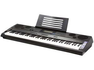 |
| Original LAION-400M alt text | Casio 76-Key Digital Keyboard Workstation (WK-6500) |
| Full caption | Black electronic keyboard with 61 white and black keys; built-in speakers on both sides; control panel with buttons and small screen above keys; detachable black music stand attached at back; plain white background. |
| Qualified object | electronic keyboard |
Example 2
| Caption type | Image / text |
|---|---|
| Image |  |
| Original LAION-400M alt text | opticalvision.co.uk |
| Full caption | Website homepage with black header featuring company logo and cat image; navigation bar with white background and black text links; central green and white advertisement banner for optical products; multiple text sections with blue and black fonts on white background; faint watermark across center. |
| Qualified object | telescope |
Example 3
| Caption type | Image / text |
|---|---|
| Image | 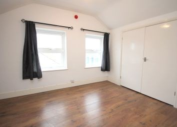 |
| Original LAION-400M alt text | Thumbnail 2 bed maisonette for sale in Shopping Centre Flats, High Street, Gorleston, Great Yarmouth |
| Full caption | Empty room with white walls and sloped ceiling; two rectangular windows with black curtains on black rods; wooden floor with warm brown tones; white double-door closet with silver handles on right wall; small red circular object above windows; white baseboard along floor; natural light entering through windows |
| Qualified object | curtain |
Full-caption training raised ObjectNet category-search mAP from 24.5 to 25.3. Qualified-object training raised it to 27.8, a gain of 3.3 points over the baseline (last column of Table 2). Richer captions are therefore less effective for the category queries tested here, although they help with richer queries. To verify this, I generated qualified object labels and full captions for a sample of 1k ObjectNet images. For each caption, I measured where its matching image ranks among those 1k images. Here I use mean reciprocal rank (MRR): average 1/rank across queries, so a match ranked first scores 1, second scores 0.5, and third scores about 0.33. This is also the metric used for training validation. In Table 2, the full-caption-trained model raises full-caption retrieval MRR from 0.700 to 0.797, compared with 0.707 for the qualified-object-trained model. The qualified-object-trained model performs best on qualified-object queries. These are ObjectNet evaluation scores; the separate LAION validation set selects the training checkpoint using a similar metric.
| Training caption type / model | Qualified object MRR | Full-caption MRR | ObjectNet mAP (%) |
|---|---|---|---|
| Baseline OpenAI-CLIP | 0.302 | 0.700 | 24.5 |
| Finetuned with full caption | 0.312 | 0.797 | 25.3 |
| Finetuned with qualified object | 0.336 | 0.707 | 27.8 |
Table 2. Training-caption style affects which queries improve most. MRR measures matching-image retrieval within the same 1k ObjectNet images; mAP measures category retrieval across the full ObjectNet gallery. Every model uses the same evaluation queries and images for each column.
Table 2: matched training settings
For Table 2, the adapted models shown start from the same OpenAI-CLIP weights and use the same 4k training images, 2k validation images and frozen image vectors. Each uses rank-16 LoRA/alpha 32, batch 128, the same learning rates, seed and stopping rule. Each model is selected by its own caption-style validation MRR.
How far can we scale this text-encoder adaptation?
Dataset size [7] and batch size [5] matter greatly during pretraining. In these adaptation experiments, however, more data yields quickly diminishing gains. Larger batches make little difference from about 1k onward, and increasing adapter rank beyond 16 provides no further improvement in the tested comparison. I hypothesize the fixed image embedding may play a role. The tables below show that validation MRR changes little across the tested batch sizes and adapter ranks. Increasing dataset size yields somewhat larger, but diminishing, gains. Higher MRR is better.
Dataset size For OpenAI-CLIP, expanding the training set from 4k to 16k images yields a smaller gain than expanding it from 1k to 4k.
| Model | 1k images | 4k images | 16k images |
|---|---|---|---|
| OpenAI-CLIP | 0.536 | 0.552 | 0.562 |
Table 3a. Validation MRR versus training-set size.
Batch size With 16k training images and a fixed adapter rank, larger batches change validation MRR little for each tested base model.
| Model | Batch 1k | Batch 2k | Batch 4k | Batch 8k |
|---|---|---|---|---|
| OpenAI-CLIP | 0.562 | 0.566 | 0.562 | 0.562 |
| OpenClip-400M | 0.602 | 0.602 | 0.604 | 0.602 |
| OpenClip-2B | — | 0.618 | 0.618 | 0.617 |
| SigLIP2 | — | 0.672 | 0.672 | — |
Table 3b. Validation MRR versus batch size. A dash marks an untested setting.
Adapter size (LoRA rank) Increasing the size of the trainable adapters also changes validation MRR little in the tested OpenAI-CLIP comparison, using 4k training images and batch size 128.
| Model | Rank 8 | Rank 16 | Rank 32 |
|---|---|---|---|
| OpenAI-CLIP | 0.545 | 0.548 | 0.546 |
Table 3c. Validation MRR versus adapter rank.
The plateau level differs by base model, as the batch-size table shows. Richer training captions do not surpass qualified-object training on ObjectNet’s simple-query MRR either (Table 2), although they help with richer queries. These are observed plateaus within the tested recipes, rather than established limits on what each model can learn. The training MRR itself continues rising.
Scaling experiments: settings and limitations
The size comparison holds LoRA rank 64, alpha 128 and batch cap 1,024 fixed across nested training sets of 1,000, 3,994 and 15,981 images, with the same 1,999 validation images. The older 4k run used a local MPS runtime and a different stopping schedule, so this is not a fully isolated test of dataset size. The batch-size comparison uses 16k training images, the same 2k validation images, and LoRA rank 64. The displayed batch sizes are rounded labels for 1,024, 2,048, 4,096 and 8,192. The adapter-size comparison uses an earlier OpenAI-CLIP 4k cohort at batch size 128; its absolute MRR should not be compared with the batch-size table as though only rank changed. All comparisons use a single training seed. Nearly identical scores do not establish statistical equivalence, and the available settings do not identify a precise threshold where returns diminish.
Could exact training-label overlap explain the gains?
Could fine-tuning help mainly because training labels repeat the category names used for evaluation? Such repetition is more likely with short object labels than with detailed captions. I grouped ObjectNet queries by whether their names appeared in the 1k training set, first appeared at 4k, or remained unmatched.
If exact label overlap were the main explanation, we would expect queries newly matched at 4k to improve more than those still unmatched. We do not see that pattern here: newly matched queries gain 0.55 mAP points, compared with 0.81 for queries that remain unmatched. This suggests the gains extend beyond learning the exact category names.
| Exact training-label overlap | Queries | Frozen OpenAI-CLIP | 1k qualified-object model | 4k qualified-object model | 4k − 1k |
|---|---|---|---|---|---|
| Already matched at 1k | 41 | 27.97 | 31.91 | 32.54 | +0.64 |
| Newly matched by 4k | 52 | 23.89 | 26.75 | 27.30 | +0.55 |
| Still unmatched at 4k | 220 | 24.01 | 26.55 | 27.36 | +0.81 |
Table 4. Retrieval improves even without exact training-label matches. ObjectNet mAP (%) for frozen OpenAI-CLIP and models trained on 1k or 4k images. Categories are grouped by when their query first matches a training label. All three groups improve over the frozen model, including queries still unmatched at 4k. The final column shows the gain from 1k to 4k in mAP points. Related labels and objects visible in training images may still contribute.
Label-overlap comparison details
A match means that a reviewed category query equals at least one of the noun variants available during training, after normalizing capitalization, punctuation and whitespace. Only training labels enter the comparison; validation labels do not. No synonym matching or word reordering is used. The three groups cover all 313 categories and are defined without looking at their AP changes.
The 1k and 4k models come from the rank-64/alpha-128, batch-cap-1,024 size comparison, with identical labels for shared images and the same 1,999 validation images. The older 4k run used a different local runtime and stopping schedule, so the comparison does not isolate dataset size completely. These are single-seed exploratory results. The frozen baseline and both adapted models use the same reviewed queries, images and relevance labels.
What does the recipe cost?
Labeling. I spent about $15 generating labels, including revisions to caption formats and prompts after inspecting the results.
Training. On Modal, the three 16k-image CLIP-family runs used for Table 1 each took about 11 minutes. The SigLIP2 run took 30 minutes; I used the checkpoint with the best validation MRR. I spent about $20 on Modal in total, including model and hyper-parameter experiments and many directions that led nowhere and are not included in this write-up.
Some related work
Cherti et al. [7] report scaling curves showing how CLIP retrieval improves with larger pretraining datasets and more compute. In one comparison holding architecture and total training examples processed fixed, expanding the pretraining dataset from 400M to 2B images raises MS-COCO image-retrieval Recall@5 from 62.3% to 65.1%. Recall@5 measures the fraction of queries whose matching image appears in the first five results; it differs from the mAP used here. [7] Their queries are full captions rather than short category names, another difference that my caption-style experiments suggest can matter. Their scaling curves nevertheless show that increasing pretraining scale improves caption retrieval.
Locked-image Tuning (LiT) trains a full text encoder against a frozen, pretrained image encoder; its large-scale setup starts the text encoder from scratch. Here, I instead adapt an existing text encoder using roughly 16k images. [10] LiT also illustrates why classification and retrieval need separate evaluation: an image encoder pretrained narrowly on ImageNet can score well on ImageNet classification yet perform worse on caption retrieval than more generally pretrained encoders. [10]
The text-image retrieval evaluations in the original CLIP paper and the OpenClip scaling study use captions from MS-COCO and Flickr30K, alongside their separate classification evaluations. [1] [7] But a search query can be a short fragment such as “electronic keyboard”, asking for relevant images rather than describing one particular image. Liu et al. [12] make a similar distinction in Flickr30K-CFQ, extending Flickr30K with compact queries, including noun phrases and entity–relation fragments. They argue that conventional caption benchmarks do not cover the range of queries used in practical search. My caption-style comparison tests how training text affects category search. I did not evaluate on Flickr30K-CFQ here, but it would be a useful next test to cover a broader range of query styles.
In SeeSaw [11], I refined CLIP’s initial query vector using relevance feedback collected during the search, without requiring a query-specific labeled training set in advance. Without the multiscale image representation, this query-refinement approach improved result quality by about 5 mAP points, averaged across LVIS, ObjectNet, COCO and BDD—three of which are also used here. [11] Those scores measure short interactive search sessions. Here, I instead adapt the text encoder beforehand using external image–text pairs, aiming to improve initial retrieval across queries and datasets before collecting query-time feedback.
Conclusion
A small, one-time adaptation of the text encoder using external images sampled from LAION-400M improved category retrieval across four models and three evaluation datasets. With roughly 16k training images, the average gain over the published prompting recipes was 4.0 points in mean average precision—similar in scale to the 3.5-point average difference between OpenClip-400M and OpenClip-2B on the same datasets. The image encoder stays fixed, so these improvements can be deployed without re-embedding an existing image collection.
The gains depend on the model and dataset, and aligning training text with the intended queries mattered more here than simply adding more data. I don’t yet know what causes these plateaus or whether a different training recipe could overcome them.
A next step could further fine-tune the adapted encoder using queries and relevance judgments collected from actual searches over the target collection. These results point to an area worth studying in detail in practice: the queries a system actually receives, including the concepts people search for, how they disambiguate them, and how much description they provide. Lightweight fine-tuning improved retrieval without requiring a new image index, making text-side adaptation a practical way to iterate on search quality in production.
Retrieval accuracy depends strongly on alignment of the caption style used for fine-tuning and the one used for querying. This means you need to iterate on the style and agree on a convention for expressing clarifications and qualifications. A system could translate users’ queries into the format used during fine-tuning, allowing people to search naturally while developers iterate on what information the retrieval model needs. This sensitivity to query style can be easy to miss when evaluation focuses on caption retrieval, as in CLIP’s MS-COCO evaluation. [1]
What I learned through these experiments
About using AI during the research process
- It is a big game changer to use AI models not only for coding, but for more parts of the research workflow, which is often more ad hoc.
- For example, generating high-quality captions with existing models enables rapid iteration on the data itself to address limitations of a particular dataset. If I want to test longer captions on a dataset that only has short ones, I can do that instead of searching for another dataset with human-generated labels of the right kind. This limitation used to block me from considering certain kinds of research directions.
- Multimodal AI tooling also made detailed error analysis easier. For example, I could identify the worst failures on ObjectNet and check how much label ambiguity affected results. It turned out not to explain most of the errors, but it did matter in this case.
- I can generate one-off interfaces to inspect labels, identify issues, and record comments. Those comments then guide AI tools when labeling or checking a larger sample. I didn’t need Jupyter notebooks at all for this project. In the past, I would have used them for tasks such as label inspection and error analysis.
- When writing, I can get very fast reading and feedback. I’m not ready yet to hand off writing to AI, but using AI during the writing process is very useful for making sentences clearer, discussing structure, and more. I haven’t yet found a good tool for collaborative writing with an AI agent of my choice.
Reaching out
I’m always interested in hearing more about Research Engineer or AI Engineer roles where I can affect the quality and cost of AI systems with my day to day work.
Reach out through LinkedIn.
Cite this post
@misc{oscarm2026clipsearch,
  author = {Moll, Oscar},
  title = {How cheaply can I improve CLIP-based image search?},
  year = {2026},
  url = {https://oscar-moll.com/blog/2026/text-encoder-adaptation/}
}
References
Links below point to the relevant sections where available. Paper-wide and notebook links are used when a reliable section link is unavailable.
-
Radford et al. (2021). Learning Transferable Visual Models From Natural Language Supervision (CLIP). Dataset construction, §2.2; encoders, §2.4; training, §2.5; prompt engineering and ensembling, §3.1.4; evaluation metrics, Table 9; few-shot and zero-shot comparison, §3.1.5; caption-retrieval evaluation, Appendix E.1.
-
OpenAI (2021). Prompt Engineering for ImageNet notebook. Published template lists and ensemble implementation. Source of the seven ImageNet-selected templates applied unchanged in my retrieval baseline.
-
Hu et al. (2021). LoRA: Low-Rank Adaptation of Large Language Models. Low-rank parameterization, §4; application to Transformers, §4.2.
-
Schuhmann et al. (2021). LAION-400M: Open Dataset of CLIP-Filtered 400 Million Image-Text Pairs. Dataset and methods, §2; filtering, §2.1.1. External source of my adaptation images and original web text.
-
Zhai et al. (2023). Sigmoid Loss for Language Image Pre-Training (SigLIP). Sigmoid-loss method, §3; batch-size experiments. Source of the pairwise sigmoid image–text objective used in my adaptation experiments.
-
Tschannen et al. (2025). SigLIP 2: Multilingual Vision-Language Encoders with Improved Semantic Understanding, Localization, and Dense Features. Architecture and text setup, §2.1; training objectives, §2.2; use as a VLM vision encoder, §3.2.
-
Cherti et al. (2023). Reproducible scaling laws for contrastive language-image learning. Retrieval scaling, §4.2; measured MS-COCO image-retrieval results, Table 21.
-
ML Foundations. OpenCLIP ImageNet prompt templates. 80-template list.
-
Hugging Face. SigLIP2 documentation. Reference inference prompt and preprocessing notes.
-
Zhai et al. (2022). LiT: Zero-Shot Transfer with Locked-image Text Tuning. Frozen-image and randomly initialized text setup, §3.3; classification evaluation, Appendix I.1; caption-retrieval evaluation, Appendix I.3.
-
Moll et al. (2023). SeeSaw: Interactive Ad-hoc Search Over Image Databases. Query-time relevance feedback and query alignment, §1; query refinement without multiscale, Table 3; publication.
-
Liu et al. (2024). Flickr30K-CFQ: A Compact and Fragmented Query Dataset for Text-image Retrieval. Caption benchmarks versus compact search queries, §1; query types and dataset construction, §3.